Quick overview
This page takes you from a fresh installation to a first measurement in a few minutes. It uses simulated instruments, so you do not need any hardware. Every step names the tab and the buttons you use; the later pages of this documentation describe each tab in detail.
What mesoscoPy does
mesoscoPy is a graphical program to run electron-transport experiments. You describe your instruments in a station file, choose which of their parameters you want to sweep and measure, and run the measurement. The data is written to QCoDeS databases, and you follow the measurement live in a plot.
Before getting started, we recommend familiarizing yourself with ‘QCoDeS <https://microsoft.github.io/Qcodes/examples/basic_examples/15_minutes_to_QCoDeS.html>’. You will need to know of QCoDeS Instruments, Parameters, Station, Measurements and Databases.
Start the program
Install mesoscoPy (see Installation), activate its environment and type:
mesoscopy
The window has six tabs, from left to right in the order you use them:
Tab |
What it is for |
|---|---|
Data |
where the data goes (database folder, sample name, logs) and the explorer of past runs |
Instruments |
load a station file and connect the instruments |
Parameter explorer |
browse the parameters of the instruments and choose the experiment parameters |
Measurement |
set up a sweep, run it and watch the live plot |
Queue |
run several measurements one after the other |
Monitor |
watch parameters over time (a temperature, a field …), with alarms |
A tab is greyed out until what it needs is there: Instruments needs a database, and the next tabs need loaded instruments. Hover over a greyed tab to read what is missing.
Try it without hardware
Download dummy.station.yaml (a station of simulated instruments) and put it in a
folder of its own, for instance Documents/mesoscopy/stations. Create another folder for the data, for instance
Documents/mesoscopy/data.
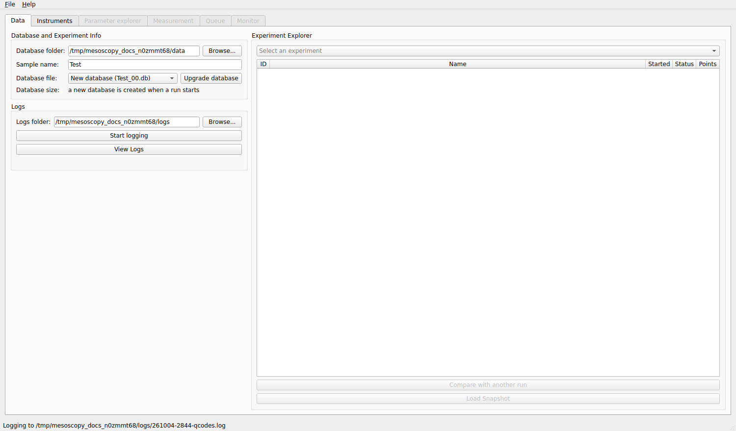
1. Data tab: say where the data goes
Under Database and Experiment Info:
click Browse… next to Database folder and choose your data folder;
type a Sample name, for example
Test.
The database is named after the sample: the first one is Test_00.db, created when the first measurement starts. (When a
database grows above 750 MB, the next measurement starts Test_01.db.) You never type a database name.
Optionally, choose a Logs folder and press Start logging to keep the QCoDeS log file there; the Monitor also writes its log in that folder.
2. Instruments tab: load the station
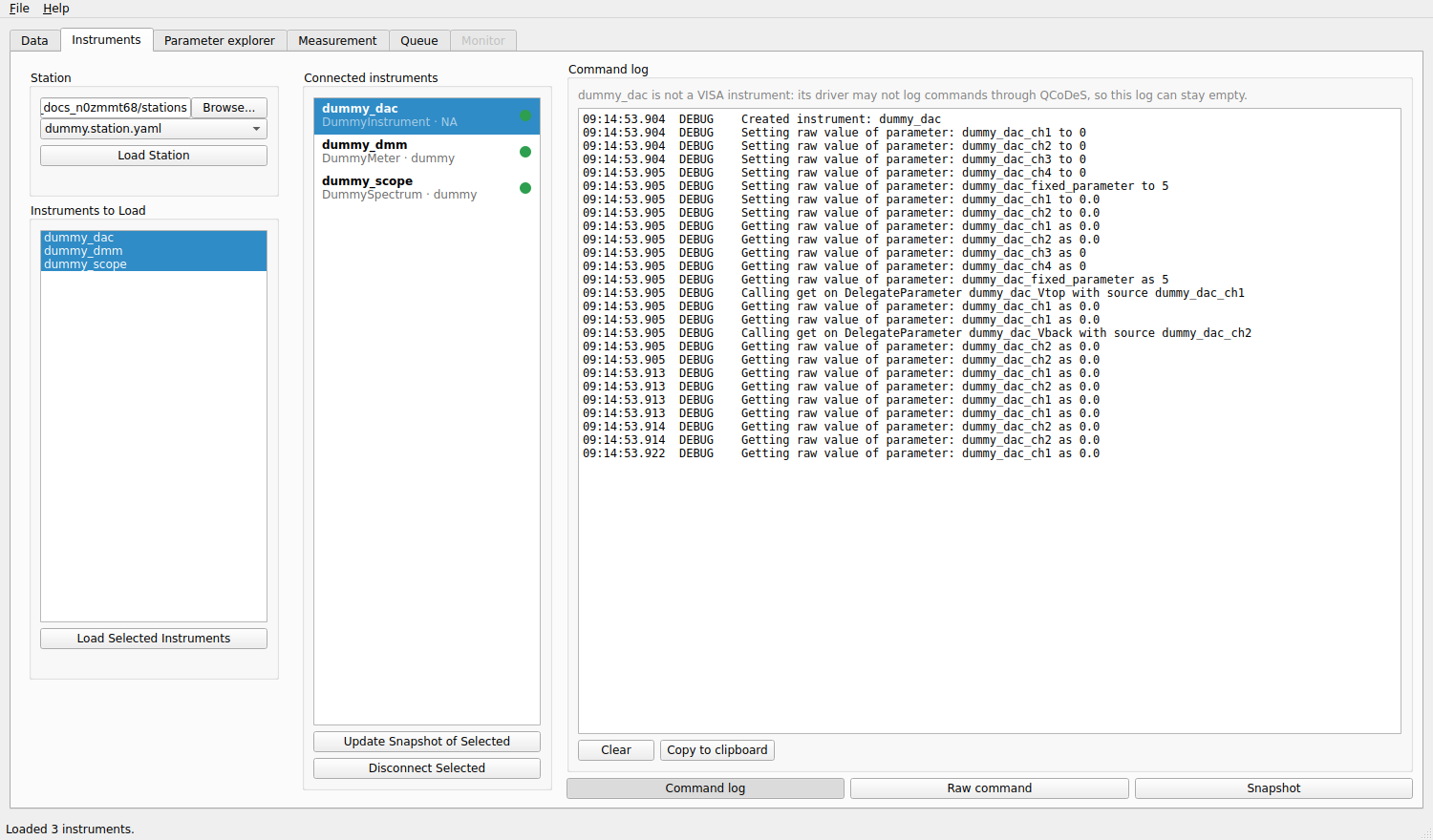
Under Station, click Browse… and choose the folder that holds dummy.station.yaml. Select the file and click
Load Station: this only reads the file. The instruments it describes appear under Instruments to Load.
Select all three (dummy_dac, dummy_dmm, dummy_scope) and click Load Selected Instruments. They move to
Connected instruments, each with a coloured dot that shows whether it answers.
3. Parameter explorer tab: the experiment parameters
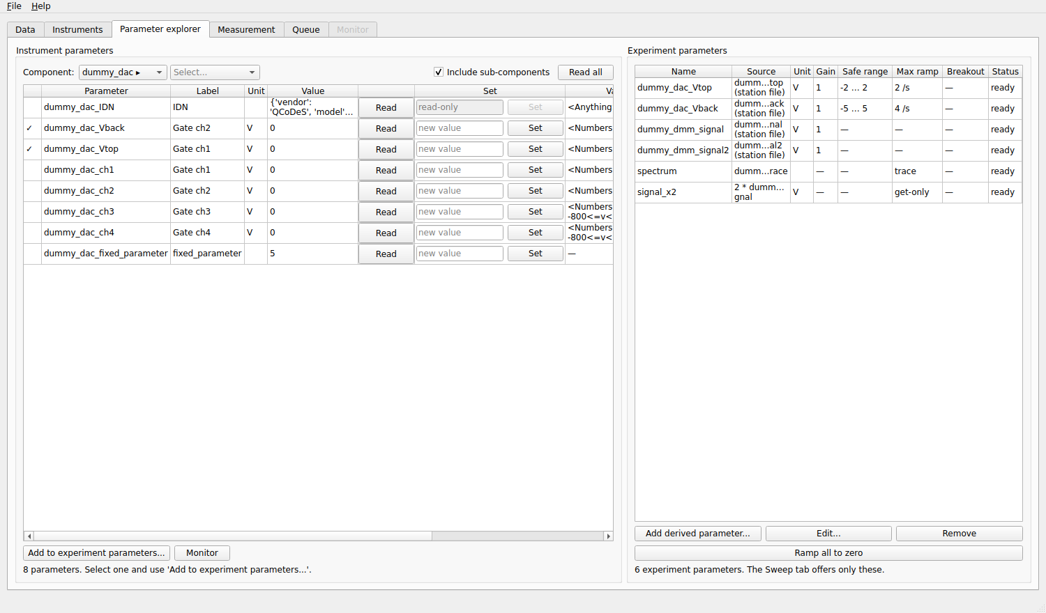
The left box, Instrument parameters, lists every parameter of the instrument you pick in Component, with its value, and lets you Read and Set it.
The right box, Experiment parameters, is the list of parameters you work with from now on. An experiment parameter has a name of your choice, an optional gain, safe limits and a maximum ramp rate; a sweep can never go beyond its limits and always moves at its ramp rate. The aliases written in the station file are already there:
dummy_dac_Vtopanddummy_dac_Vback: the two gates, limited to ±2 V and ±5 V;dummy_dmm_signalanddummy_dmm_signal2: two readings that follow the gates.
To make another instrument parameter an experiment parameter, select it on the left and click Add to experiment parameters…. Add derived parameter… makes a computed one, such as a density, from other experiment parameters.
Note
Set the safe limits and the ramp rates of the gates before you connect a real sample. They are what protects it.
4. Measurement tab: sweep and measure
Give the measurement a Measurement name, for example
first sweep: the Run button stays disabled until it has one. Experiment Name groups related measurements in the database; if you leave it empty the experiment is calledSweep.In the Sweep box leave the class on LinSweep, choose
dummy_dac_Vtopas the Sweep component, and enter Start-1, Stop1, Num points101and Delay (s)0.01(the time to wait at each point).Under Measured Parameters click Add parameter… and add
dummy_dmm_signal.
Click Check setup to see what the measurement will do before it starts: it checks the sweep against the safe limits and reports the estimated duration without touching an instrument. Then click Run.
The plot on the right follows the run: the elapsed and remaining times are above it, the X axis and Y axis selectors
below let you plot any swept or measured parameter, and the faded curves are the earlier runs. You should see a peak
centred on Vtop = 0.
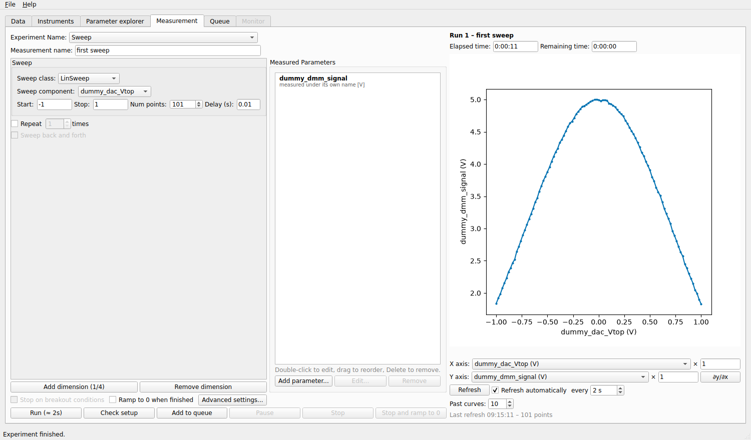
Pause stops after the current point, Stop ends the run cleanly (what was written stays), and Stop and ramp to 0 also brings the swept parameters back to 0.
5. Data tab: find the run again
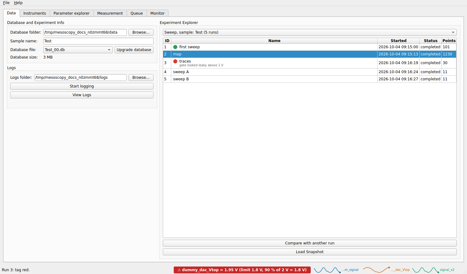
Back in the Data tab, the Experiment Explorer lists the experiments and the runs of the database. Right-click a run to give it a colour tag or notes, to compare it with another run, or to load its snapshot.
Where to go next
Sweeps of two or more parameters, repetitions, traces and the Advanced settings…: Measurement tab.
The parameters you work with, their safe limits and ramp rates: Parameter explorer tab.
Several measurements one after the other, waits and series: Queue tab.
Watching a temperature or a field over time, and alarms: Monitor tab.
Describing your own instruments in a station file: Building the station file, and connecting them: Instruments tab.
Safe limits, ramp rates and what happens when you close the program: Safety.
Program-wide options (File, Settings…): Settings and About.
What the program does not do yet: Limitations and roadmap.